0%

在去年曾经tutor过一些数学竞赛,很多题目有关一个数除x余y, 然后求这个数是多少的。

比如 一个数当除以3余2,除以5余3,除以7余2,那么这个数是多少

x = 2 mod 3

x = 3 mod 5

x = 2 mod 7

这个时候分成3个mod 部分分别求基础解。

比如第一部分 另外两个mod的乘积为 5 x 7 = 35

然后在mod 3 中求 35 的倒数

35 x 2 = 1 mod 3

再把 倒数 x 一开始余的数 x 另外两个mod 的乘积 = 2 x 2 x 35 = 140

然后同理,求出另外两个mod的结果再加在一起 = 233,

那么所有233 + (3x5x7) x k 的数都满足这个条件

接下来我想尝试写一个python 程序解决所有诸如此类的问题

1
2
3
4
5
6
7
8
9
10
11
12
13
14
15
16
17
18
19
20
21
22
23
24
25
def inverseMod(number, mod):
total = 1
for i in range(mod):
if (total%number) == 0:
return total/number
total = total + mod
return False

def chineseRemainingTheory(remainList, modList):
inverserModList = []
allProduct = 1
for i in modList:
allProduct = allProduct * i
result = 0
for index in range(len(remainList)):
products = (allProduct/modList[index])
inverse = inverseMod(products%modList[index], modList[index])
result = result + (inverse * products * remainList[index])
return result

def main():
remainList = [2,3,2]
modList = [3,5,7]
result = chineseRemainingTheory(remainList, modList)
print (result, "should = 233")

变性之差一段DNA

30 年前就有一支生物团队发现一段Sry 基因,可以使雌性小白鼠发育成雄性。

最近有新的进展发现Sry 基因可以控制合成SOX9的蛋白,动物会在这段蛋白的影响下发育出雄性的生殖器官。

反之如果雄性缺少这段蛋白也能变成雌性。

Reference:

(Evidence to exclude SOX9 as a candidate gene for XY sex reversal without skeletal malformation)[http://jmg.bmj.com/content/jmedgenet/33/9/800.full.pdf]

非双螺旋的新DNA结构

新的结构命名为“i-motif”, 类似于结。研究人员发现i-motif-随着时间的推移而出现和消失,所以它们正在形成,溶解并再次形成。

I-基序(i-motif) 可能帮助开启或关闭基因,并影响基因是否被主动读取。

另外一种天然的结构

G四联体(G quadruplex,又称G-tetrads或G4-DNA)

其中研究较为深入的区域,是染色体末端的端粒(telomere)。

(DNA可不只有双螺旋结构)[https://zhuanlan.zhihu.com/p/36216255]

反向传播

Introduction:

反向传播是利用链式法则递归计算表达式的梯度的方法。 根据函数 f(x), 求关于f 关于 x的梯度 gradient

偏导数

(我的理解就是当对其中一个param 求导的时候视其他的params为const, 含义为当这个param 增加的时候 对f 的增加量的比值)

链式法则

Chain rule

这下面这个sample给的真的是清楚

x = -2; y = 5; z = -4

f(x,y,z) = (x+y)z

绿色的从输入端到输出端 为前向传播

红色的从输出端到输入端 为反向传播

反向传播的理解

反向传播是一个优美的局部过程。在整个计算线路图中,每个门单元都会得到一些输入并立即计算两个东西:

1.这个门的输出值,

2.其输出值关于输入值的局部梯度。

门单元完成这两件事是完全独立的,它不需要知道计算线路中的其他细节。然而,一旦前向传播完毕,在反向传播的过程中,门单元门将最终获得整个网络的最终输出值在自己的输出值上的梯度。链式法则指出,门单元应该将回传的梯度乘以它对其的输入的局部梯度,从而得到整个网络的输出对该门单元的每个输入值的梯度。

因为在加法门中 是 y = a+b 所以slope 也就是梯度都是1, 在乘法门中 y = ab, 所以a 的梯度就是b, b的梯度就是a

Example

w = [2,-3,-3] # 假设一些随机数据和权重
x = [-1, -2]

# 前向传播
dot = w[0]*x[0] + w[1]*x[1] + w[2]
f = 1.0 / (1 + math.exp(-dot)) # sigmoid函数

# 对神经元反向传播
ddot = (1 - f) * f # 点积变量的梯度, 使用sigmoid函数求导
dx = [w[0] * ddot, w[1] * ddot] # 回传到x
dw = [x[0] * ddot, x[1] * ddot, 1.0 * ddot] # 回传到w
# 完成!得到输入的梯度

Tip:

对前向传播变量进行缓存:在计算反向传播时,前向传播过程中得到的一些中间变量非常有用。在实际操作中,最好代码实现对于这些中间变量的缓存,这样在反向传播的时候也能用上它们。如果这样做过于困难,也可以(但是浪费计算资源)重新计算它们。

在不同分支的梯度要相加:如果变量x,y在前向传播的表达式中出现多次,那么进行反向传播的时候就要非常小心,使用+=而不是=来累计这些变量的梯度(不然就会造成覆写)。这是遵循了在微积分中的多元链式法则,该法则指出如果变量在线路中分支走向不同的部分,那么梯度在回传的时候,就应该进行累加。 比如 f(x,y) = sigmal(x) + x balabala

回传流中的模式

主要就是

加法门单元: 把输出的梯度相等地分发给它所有的输入,这一行为与输入值在前向传播时的值无关。这是因为加法操作的局部梯度都是简单的+1,所以所有输入的梯度实际上就等于输出的梯度,因为乘以1.0保持不变。上例中,加法门把梯度2.00不变且相等地路由给了两个输入。

y = 1.0 x a + 1.0 x b

取最大值门单元: 对梯度做路由。和加法门不同,取最大值门将梯度转给其中一个输入,这个输入是在前向传播中值最大的那个输入。这是因为在取最大值门中,最高值的局部梯度是1.0,其余的是0。上例中,取最大值门将梯度2.00转给了z变量,因为z的值比w高,于是w的梯度保持为0。

y = max(high, low) = 1.0 x high + 0 x low

乘法门单元: 相对不容易解释。它的局部梯度就是输入值,但是是相互交换之后的,然后根据链式法则乘以输出值的梯度。上例中,x的梯度是-4.00x2.00=-8.00。

y = ab, a的梯度是b

用向量化操作计算梯度

其实就是矩阵相乘之类,作者建议通过维度来推测计算是否正确

Summary:

对梯度的含义有了直观理解,知道了梯度是如何在网络中反向传播的,知道了它们是如何与网络的不同部分通信并控制其升高或者降低,并使得最终输出值更高的。(梯度如何计算)

讨论了分段计算在反向传播的实现中的重要性。应该将函数分成不同的模块,这样计算局部梯度相对容易,然后基于链式法则将其“链”起来。重要的是,不需要把这些表达式写在纸上然后演算它的完整求导公式,因为实际上并不需要关于输入变量的梯度的数学公式。只需要将表达式分成不同的可以求导的模块(模块可以是矩阵向量的乘法操作,或者取最大值操作,或者加法操作等),然后在反向传播中一步一步地计算梯度。(不难理解,但是不知道实际操作是否需要,我感觉每一层都会有自己计算梯度的方法)

Reference:

反向传播

Sequlize cli 是一个后端对象控制的一个library

Introduce

首先要install: npm install –save sequelize-cli

然后init: node_modules/.bin/sequelize init

如果你是用Mac 你可以重命名 sequelize: alias sequelize=’node_modules/.bin/sequelize’

设置 config/config.json 基本上就是列出 database的schema username password 之类的

Migration

一种是create migration by model

node_modules/.bin/sequelize model:generate --name User

还有一种是直接create migration

node_modules/.bin/sequelize migration:create --name add-wechatid-in-user

Seed

在数据库里生成一些demo 或者 测试dat啊

生成 demo-user 的 seed

node_modules/.bin/sequelize seed:generate --name demo-user

在seeder 文件里

'use strict';
module.exports = {
  up: (queryInterface, Sequelize) => {
    return queryInterface.bulkInsert('Users', [{
        firstName: 'John',
        lastName: 'Doe',
        email: 'demo@demo.com'
      }], {});
  },

  down: (queryInterface, Sequelize) => {
    return queryInterface.bulkDelete('Users', null, {});
  }
};

Reference:

Sequelize 手册

Review

  • 基于参数的评分函数。该函数将原始图像像素映射为分类评分值。

  • 损失函数。该函数能够根据分类评分和训练集图像数据实际分类的一致性,衡量某个具体参数集的质量好坏。损失函数有多种版本和不同的实现方式(例如:Softmax或SVM)。 Softmax 和 SVM 不应该包括了score function 和 lost function

  • 最优化Optimization。最优化是寻找能使得损失函数值最小化的参数W的过程。

损失函数可视化

  • 在一维尺度上 $$L(W+aW_1)$$ x轴是a, y轴是loss function

  • 在二维尺度上 $$L(W+aW_1+bW_2)$$, a,b 表达x轴, y轴, loss function 用颜色表示

单独的损失函数表示:

$$w_j$$ 如果对应分类正确即是负号,错误即是正号 $$L = \sumL/n$$

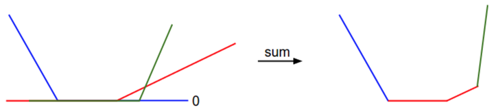
SVM的损失函数是一种凸函数,可以学习一下如何高效最小化凸函数,在这种损失函数会有一些不可导的点(kinks)

两个新概念:

  • 梯度? 次梯度?未来学习点

最优化 Optimization

对于神经网络的最优化策略有:

策略#1:随即搜索 最差劲的搜索方案(base line)

# 假设X_train的每一列都是一个数据样本(比如3073 x 50000)
# 假设Y_train是数据样本的类别标签(比如一个长50000的一维数组)
# 假设函数L对损失函数进行评价

bestloss = float("inf") # Python assigns the highest possible float value
for num in xrange(1000):
  W = np.random.randn(10, 3073) * 0.0001 # generate random parameters
  loss = L(X_train, Y_train, W) # get the loss over the entire training set
  if loss < bestloss: # keep track of the best solution
    bestloss = loss
    bestW = W
  print 'in attempt %d the loss was %f, best %f' % (num, loss, bestloss)

感觉跟那个monkey sort 差不多 随机生成W weight。

# 假设X_test尺寸是[3073 x 10000], Y_test尺寸是[10000 x 1]
scores = Wbest.dot(Xte_cols) # 10 x 10000, the class scores for all test examples
# 找到在每列中评分值最大的索引(即预测的分类)
Yte_predict = np.argmax(scores, axis = 0)
# 以及计算准确率
np.mean(Yte_predict == Yte)
# 返回 0.1555

策略是:随机权重开始,然后迭代取优,从而获得更低的损失值。

策略#2:随机本地搜索

生成一个随机的扰动 $$ \delta W $$

$$ Wtry = W + \delta W $$

当 Wtry 的loss 变小的时候, 才决定移动

W = np.random.randn(10, 3073) * 0.001 # 生成随机初始W
bestloss = float("inf")
for i in xrange(1000):
  step_size = 0.0001
  Wtry = W + np.random.randn(10, 3073) * step_size
  loss = L(Xtr_cols, Ytr, Wtry)
  if loss < bestloss:
    W = Wtry
    bestloss = loss
  print 'iter %d loss is %f' % (i, bestloss)
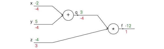
策略#3:跟随梯度

策略1 和 策略2 都是尝试好几个方向来找减少loss的方向,其实可以用梯度(gradient)来找到最陡峭的方向减少loss,

一维求导公式: d(fx)/dx

当函数有多个参数的时候,我们称导数为偏导数。而梯度就是在每个维度上偏导数所形成的向量。

梯度计算

有两种方法计算梯度:

数值梯度法 (实现简单 但是缓慢)

def eval_numerical_gradient(f, x):
  """  
  一个f在x处的数值梯度法的简单实现
  - f是只有一个参数的函数
  - x是计算梯度的点
  """ 

  fx = f(x) # 在原点计算函数值
  grad = np.zeros(x.shape)
  h = 0.00001

  # 对x中所有的item索引进行迭代
  it = np.nditer(x, flags=['multi_index'], op_flags=['readwrite'])
  while not it.finished:

    # 计算x+h处的函数值
    ix = it.multi_index
    old_value = x[ix]
    x[ix] = old_value + h # 增加h
    fxh = f(x) # 计算f(x + h)
    x[ix] = old_value # 存到前一个值中 (非常重要)

    # 计算偏导数
    grad[ix] = (fxh - fx) / h # 坡度
    it.iternext() # 到下个维度

  return grad

实际中用中心差值公式(centered difference formula)[f(x+h)-f(x-h)]/2h 效果较好 Numerical_differentiation

# 要使用上面的代码我们需要一个只有一个参数的函数
# (在这里参数就是权重)所以也包含了X_train和Y_train
def CIFAR10_loss_fun(W):
  return L(X_train, Y_train, W)

W = np.random.rand(10, 3073) * 0.001 # 随机权重向量
df = eval_numerical_gradient(CIFAR10_loss_fun, W) # 得到梯度

loss_original = CIFAR10_loss_fun(W) # 初始损失值
print ‘original loss: %f’ % (loss_original, )

# 查看不同步长的效果
for step_size_log in [-10, -9, -8, -7, -6, -5,-4,-3,-2,-1]:
  step_size = 10 ** step_size_log
  W_new = W - step_size * df # 权重空间中的新位置
  loss_new = CIFAR10_loss_fun(W_new)
  print 'for step size %f new loss: %f' % (step_size, loss_new)

# 输出:
# original loss: 2.200718
# for step size 1.000000e-10 new loss: 2.200652
# for step size 1.000000e-09 new loss: 2.200057
# for step size 1.000000e-08 new loss: 2.194116
# for step size 1.000000e-07 new loss: 2.135493
# for step size 1.000000e-06 new loss: 1.647802
# for step size 1.000000e-05 new loss: 2.844355
# for step size 1.000000e-04 new loss: 25.558142
# for step size 1.000000e-03 new loss: 254.086573
# for step size 1.000000e-02 new loss: 2539.370888
# for step size 1.000000e-01 new loss: 25392.214036

步长的影响:梯度指明了函数在哪个方向?是变化率最大的 步长(也叫作学习率)

小步长下降稳定但进度慢 <-> 大步长进展快但是风险更大

在本例中有30730个参数,所以损失函数每走一步就需要计算30731次损失函数的梯度, 效率太低

分析梯度法 (计算迅速,结果精确) 微分分析计算梯度

用公式计算梯度速度很快,唯一不好的就是实现的时候容易出错. 于是我们需要将分析梯度法的结果于数值梯度法作比较, 这个步骤叫做梯度检查。

eg: SVM lossfunction

对W_yi 进行微分

梯度下降

普通版本

# 普通的梯度下降
while True:
  weights_grad = evaluate_gradient(loss_fun, data, weights)
  weights += - step_size * weights_grad # 进行梯度更新

小批量数据梯度下降(Mini-batch gradient descent)

每次小子集往下减少,小批量数据的梯度就是对整个数据集梯度的一个近似, 需要data的数量远大于小批数量

# 普通的小批量数据梯度下降
while True:
  data_batch = sample_training_data(data, 256) # 256个数据
  weights_grad = evaluate_gradient(loss_fun, data_batch, weights)
  weights += - step_size * weights_grad # 参数更新

随机梯度下降(Stochastic Gradient Descent 简称SGD)

如果小批量数据中每个批量只有1个数据样本

Summary:

x,y 是给定的,weight 从一个随机开始,可以随时改变。 损失函数包含两个部分:数据损失和正则化损失,在梯度下降中,计算权重的维度实现参数的更新。

Reference:

最优化上

最优化下

Pyenv

因为之前用nvm node 的版本管理器

所以pyenv 应该也是python 的版本管理器

运行 curl -L https://github.com/pyenv/pyenv-installer/raw/master/bin/pyenv-installer | bash

然后打开 vim ~/.bash_profile

添加了三行

export PATH="~/.pyenv/bin:$PATH"
eval "$(pyenv init -)"
eval "$(pyenv virtualenv-init -)"

我原来的是

export XAMPP_HOME=/Applications/xampp/xamppfiles
export PATH=${XAMPP_HOME}/bin:${PATH}

最后变成

export XAMPP_HOME=/Applications/xampp/xamppfiles
export PATH=/Users/weijiesun/.pyenv/bin:${PATH}:${XAMPP_HOME}/bin

eval "$(pyenv init -)"
eval "$(pyenv virtualenv-init -)"

然后有个坑踩了好久,就是XAMPP_HOME=/Applications/xampp/xamppfiles 要放在path 的最后一位,不然就是疯狂在找http url 的端口

然后运行

source ~/.bash_profile     

就好了

Cheating sheet:reference

  • 安装和查看pyenv 和 python

    #查看pyenv版本
    pyenv –version

    #查看可用的python version
    pyenv versions

    #用pyenv 安装python
    pyenv install 3.6.3

  • 设置 python version

    对所有的Shell全局有效,会把版本号写入到~/.pyenv/version文件中

    pyenv global 3.6.3

    只对当前目录有效,会在当前目录创建.python-version文件

    pyenv local 3.6.3

    只在当前会话有效

    pyenv shell 3.6.3

我在安装的时候遇到了一下描述的问题

Last 10 log lines:   File "/private/var/folders/py/3006ng_x6x3g5c42jx_gznlc0000gn/T/python-build.20180618223416.3806/Python-3.6.3/Lib/ensurepip/__main__.py", line 4, in <module>     ensurepip._main()

解决方法

Kears

# GPU 版本
>>> pip install --upgrade tensorflow-gpu

# CPU 版本
>>> pip install --upgrade tensorflow

# Keras 安装
>>> pip install keras -U --pre

import keras
#然后就显示tensorflow work on backend

pyecharts

github pyecharts

1
2
3
4
5
6
7
8
$ pip install pyecharts


$ pip install echarts-countries-pypkg
$ pip install echarts-china-provinces-pypkg
$ pip install echarts-china-cities-pypkg
$ pip install echarts-china-counties-pypkg
$ pip install echarts-china-misc-pypkg

$ pip install echarts-united-kingdom-pypkg

Reference:

https://zhuanlan.zhihu.com/p/20918580

https://zhuanlan.zhihu.com/p/20945670

https://zhuanlan.zhihu.com/p/21102293

Linear Classification

score function (评分函数)

原始图片到各个类别的评分情况, 分越高越接近

每个图像都是 [D x 1] D = pixel X pixel X 3(RGB)

参数

权重

W (weight) = [k X D] k是样本数

在维度空间里 做旋转变换

偏差向量

b (bias vector) = [k x 1]

在维度空间里 做平移变化

图像数据预处理

最常见的就是 normalization

零均值的中心化 把 [0-255] -> [-127-127] -> [-1,1]

Loss Function (损失函数)

量化分类label 与真实label 之间的一致性 也叫 代价函数Cost Function或目标函数Objective

当 Score Function 与真实结果相差越大,Cost Function输出越大

多类支持向量机损失 Multiclass Support Vector Machine Loss

eg: 有三个分类 score 是 s = [13, -7, 11] \delta = 10, 第一个label 是真实正确的

因为 -20 大于 \delta 边界值, 所以最后的损失值为8

线性评分函数 的损失函数公式:

折叶损失(hinge loss): max (0, -)

平方折叶损失SVM(即L2-SVM): max (0, -) ^2

目的是想要正确类别进入红色区域, 如果其他类别进入红色区域甚至更高的时候,计算loss, 我们的目的是找权重W

Regularization 正则化

假设有一个数据集和一个权重集W能够正确地分类每个数据, 可能有很多相似的W都能正确地分类所有的数据

比如有一个权重W 调整系数可以改变Loss score。 我们希望給W添加一些偏好

向损失函数增加一个正则化惩罚

egularization penalty 正则化惩罚 R(W)

多类SVM损失函数 L = 数据损失(data loss),即所有样例的的平均损失L_i + 正则化损失(regularization loss)

展开公式

Code:

def L_i(x, y, W):
  """
  unvectorized version. Compute the multiclass svm loss for a single example (x,y)
  - x is a column vector representing an image (e.g. 3073 x 1 in CIFAR-10)
    with an appended bias dimension in the 3073-rd position (i.e. bias trick)
  - y is an integer giving index of correct class (e.g. between 0 and 9 in CIFAR-10)
  - W is the weight matrix (e.g. 10 x 3073 in CIFAR-10)
  """
  delta = 1.0 # see notes about delta later in this section
  scores = W.dot(x) # scores becomes of size 10 x 1, the scores for each class
  correct_class_score = scores[y]
  D = W.shape[0] # number of classes, e.g. 10
  loss_i = 0.0
  for j in xrange(D): # iterate over all wrong classes
    if j == y:
      # skip for the true class to only loop over incorrect classes
      continue
    # accumulate loss for the i-th example
    loss_i += max(0, scores[j] - correct_class_score + delta)
  return loss_i

def L_i_vectorized(x, y, W):
  """
  A faster half-vectorized implementation. half-vectorized
  refers to the fact that for a single example the implementation contains
  no for loops, but there is still one loop over the examples (outside this function)
  """
  delta = 1.0
  scores = W.dot(x)
  # compute the margins for all classes in one vector operation
  margins = np.maximum(0, scores - scores[y] + delta)
  # on y-th position scores[y] - scores[y] canceled and gave delta. We want
  # to ignore the y-th position and only consider margin on max wrong class
  margins[y] = 0
  loss_i = np.sum(margins)
  return loss_i

def L(X, y, W):
  """
  fully-vectorized implementation :
  - X holds all the training examples as columns (e.g. 3073 x 50,000 in CIFAR-10)
  - y is array of integers specifying correct class (e.g. 50,000-D array)
  - W are weights (e.g. 10 x 3073)
  """
  # evaluate loss over all examples in X without using any for loops
  # left as exercise to reader in the assignment
    delta = 1.0
    score_matrix = W.dot(X)
    correct_score = score_matrix[y]
    #Todo, correct_score_matrix = correct_core * 50
    #Todo, delta_matrx repeat delta
    loss_matrix = score_matrix - correct_score_matrix + delta_matrx
    result = np.sum(loss_matrix, axis=1)
  return loss_matrix

Softmax分类器

逻辑回归分类器面对多个分类的一般化归纳

公式:

或者

所有的函数转换成 $$e^z$$

score function =>

softmax 函数, 每个元素都在0-1之间并且和为1

概率解释:

我们就是在最小化正确分类的负对数概率,这可以看做是在进行最大似然估计(MLE)

实现softmax函数计算的时候技巧可以用常数C, 通常$$\log C = -maxf_j$$

f = np.array([123, 456, 789]) # 例子中有3个分类,每个评分的数值都很大
p = np.exp(f) / np.sum(np.exp(f)) # 不妙:数值问题,可能导致数值爆炸

# 那么将f中的值平移到最大值为0:
f -= np.max(f) # f becomes [-666, -333, 0]
p = np.exp(f) / np.sum(np.exp(f)) # 现在OK了,将给出正确结果

折叶损失(hinge loss)替换为交叉熵损失(cross-entropy loss)

SVM和Softmax的比较

Softmax

Summary

  • SVM 和 Softmax 基于 weight W 和 bias b

  • define Loss Function (损失函数) 用来更好的定义更好的预测模型

—-sad—-
Test Mathjax, 但是公式实在太复杂。

$$
L{i}=f{yi}+\log (\sum{j} e^{f_j})
$$

$L_{i} = -\log \frac {e^{f_y}} {e^{f_j}}$

$\sum_{j=0}$

$$
a+b=c
$$

TODO

Reference:

https://zhuanlan.zhihu.com/p/20894041

https://zhuanlan.zhihu.com/p/20900216

图像分类

颜色channel 有三个 red green blue, RGB

流程就是 输入 -> 学习 -> 评价

K Nearest Neighbor 分类器

k 越高 generalization 能力越好

用距离来分类

L1范数 和 L2范数

L1

L2

distances = np.sqrt(np.sum(np.square(self.Xtr - X[i,:]), axis = 1))

L1和L2比较。。在面对两个向量之间的差异时,L2比L1更加不能容忍这些差异。也就是说,相对于1个巨大的差异,L2距离更倾向于接受多个中等程度的差异。L1和L2都是在p-norm常用的特殊形式。

hyperparameter: 超参数,需要去测试调整

validation set: 测试集 只能使用一次

Cross validation: train <-> test

##k Nearest Neighbor 优缺点:

Advantange:易于理解,实现简单。

Disadvantage: 算法的训练不需要花时间,因为其训练过程只是将训练集数据存储起来。然而测试要花费大量时间计算,因为每个测试图像需要和所有存储的训练图像进行比较,这显然是一个缺点。在实际应用中,我们关注测试效率远远高于训练效率

Reference: https://zhuanlan.zhihu.com/p/36287950

Todo List

  • [X] - 01 - Overview
    P1-15 Machine learning background and flow

P16-42 Machine learning flow

  • [ ] - 02 - Business Understanding

  • [X] - 03 - Data Understanding p56 - 62

    To learn about data analysis, it is right that each of us try many things that do not work – that we tackle more problems than we make expert analyses of. We often learn less from an expertly done analysis than from one where, by not trying something, we missed an opportunity to learn more

  • [ ] - 04 - Data Preparation -p63

Prepare data is time consuming

several methods to deal with missing data and outliers

normalize Data

Data binning 分级

Reduce Data, Clean Data

Feature Engineering: 从raw data 提取出 feature

Feature Selection: Filter/Wrapper/Embedded method

Traditional approaches 传统方法

Forward selection

一开始模型里面没有variable, 然后往里面加入variable,直到accuracy 没有任何的增长

Backward elimination

和前一种相反,一开始有所有的variable, 然后去除,直到accuracy 有明显的下降

Stepwise regression

这种是用在选k-best feature, 一开始有k个,然后加入更好的,并且去除最差的,直到经历过所有的feature

P100

Containers

List Containers

docker ps (show all the running container)

docker ps -a (show all the container include which is not running)

Start container

docker start {containerId} (start one container)

Stop container

docker stop {containerId} (Stop one container)

Docker-Compose

Create a docker-compose.yml document

To be continue